14.2.5. Nonlinear MDOF
The source code is developed by Joseph Jaramillo from National University of Engineering.
The source code is shown below, which can be downloaded
here.The ground motion file
here.And also the python plotting script
here.Make sure the numpy and matplotlib packages are installed in your Python distribution.
Run the source code in your favorite Python program and should see:
Natural periods:       Natural frequencies:
T1 = 0.628 [s]    |    f1 = 1.592 [Hz]
T2 = 0.257 [s]    |    f2 = 3.898 [Hz]
T3 = 0.162 [s]    |    f3 = 6.164 [Hz]
1'''
2=========================================================================================================================
3================================================== NonLinear MDOF =======================================================
4=========================================================================================================================
5
6By M. Eng. Joseph Jaramillo, National University of Engineering
7e-mail: jjaramillod@uni.edu.pe
8Date - 22/10/2024
9
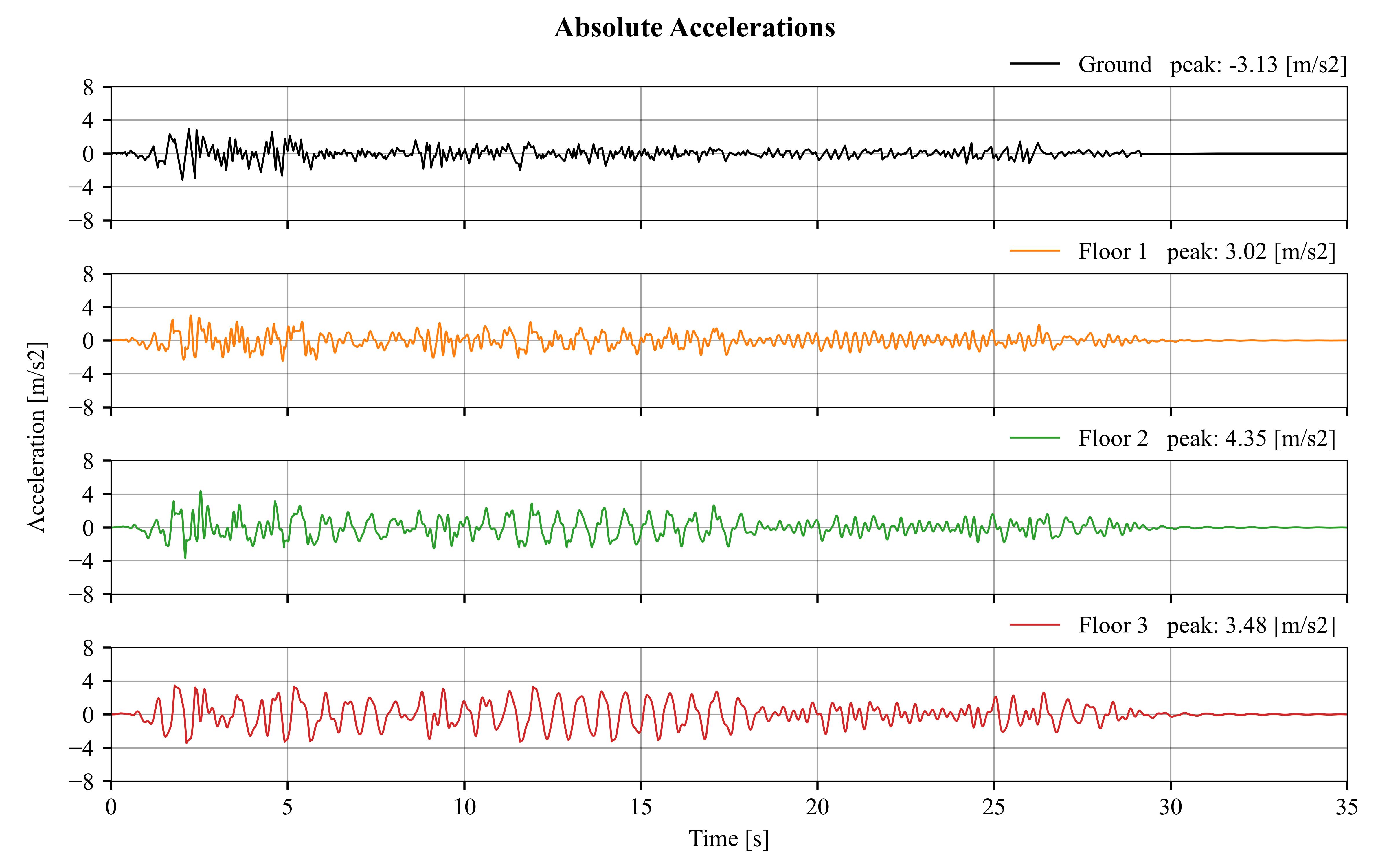
10This example models a multi-degree-of-freedom (MDOF) damped system commonly used in earthquake engineering of a three-story
11building. It conducts a nonlinear dynamic (time history) analysis using the El Centro 1940 earthquake as the input ground
12motion.
13'''
14
15import openseespy.opensees as ops
16import numpy as np
17import plot_nonlinear_mdof_graphs
18# Base units
19m = 1 # Meters
20s = 1 # Seconds
21kN = 1 # Kilo Newtons
22
23# Derivated units
24g = 9.81*m/s**2 # Gravity
25cm = 1e-2*m # Centimeter
26mm = 1e-3*m # Milimeter
27Ton = kN*s**2/m # Ton
28
29# Parameters - data
30N = 3 # N° DOF
31h = 0.05 # Damping ratio
32dt = 0.02 # Time step
33dt_out = 0.001 # Output time step
34tFinal = 35 # Analysis stop time
35m1 = 0.1*Ton # Mass / floor
36m2 = 0.1*Ton
37m3 = 0.1*Ton
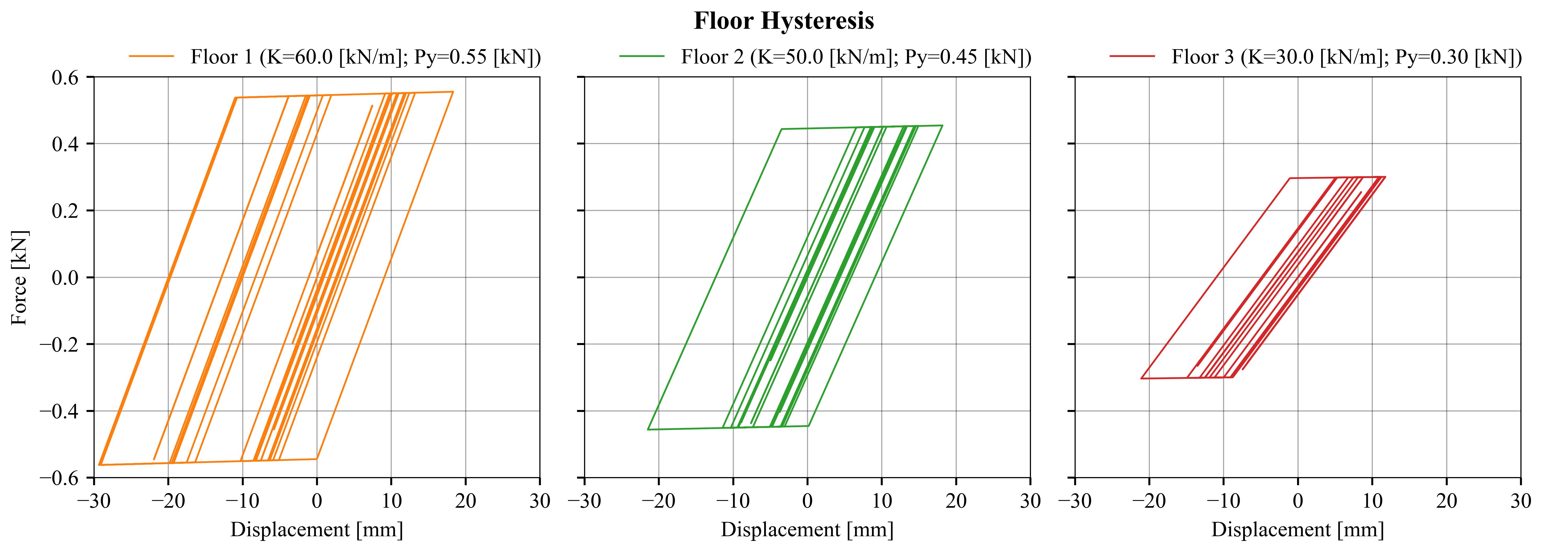
38Py1 = 0.55*kN # Yielding strength / floor
39Py2 = 0.45*kN
40Py3 = 0.30*kN
41K1 = 60*kN/m # Stiffness / floor
42K2 = 50*kN/m
43K3 = 30*kN/m
44b = 0.01 # Strain-hardening ratio
45
46######## Model ###############
47ops.wipe() # clear memory of all past model definitions
48ops.model('basic', '-ndm', 1, '-ndf', 1) # Define the model builder, ndm=#dimension, ndf=#dofs
49
50# Create nodes
51ops.node(0, 0)
52ops.node(1, 0, '-mass', m1)
53ops.node(2, 0, '-mass', m2)
54ops.node(3, 0, '-mass', m3)
55
56# Define boundary condition
57ops.fix(0, 1)
58
59# Material definition
60ops.uniaxialMaterial('Steel01', 1, Py1, K1, b)
61ops.uniaxialMaterial('Steel01', 2, Py2, K2, b)
62ops.uniaxialMaterial('Steel01', 3, Py3, K3, b)
63
64# Element definition
65ops.element('zeroLength', 1, 0, 1, '-mat', 1 , '-dir', 1, '-doRayleigh', 1)
66ops.element('zeroLength', 2, 1, 2, '-mat', 2 , '-dir', 1, '-doRayleigh', 1)
67ops.element('zeroLength', 3, 2, 3, '-mat', 3 , '-dir', 1, '-doRayleigh', 1)
68
69# Set Rayleigh damping
70w1, w2, w3 = np.array(ops.eigen('-fullGenLapack', 3))**0.5
71a0 = 2*h*w1*w2/(w1+w2)
72a1 = 2*h/(w1+w2)
73ops.rayleigh(a0, .0, .0, a1) # RAYLEIGH damping
74
75# Natural periods
76print('\nNatural periods: Natural frequencies:')
77print(f'T1 = {2*np.pi/w1:.3f} [s] | f1 = {w1/(2*np.pi):.3f} [Hz]')
78print(f'T2 = {2*np.pi/w2:.3f} [s] | f2 = {w2/(2*np.pi):.3f} [Hz]')
79print(f'T3 = {2*np.pi/w3:.3f} [s] | f3 = {w3/(2*np.pi):.3f} [Hz]')
80
81# Define the dynamic analysis
82load_tag = 1
83patter_tag = 1
84direc = 1
85ops.timeSeries('Path', load_tag, '-dt', dt, '-filePath', r'./el_centro.th', '-factor', g) # Reading ground motion
86ops.pattern('UniformExcitation', patter_tag, direc, '-accel', load_tag)
87
88# Define output data files
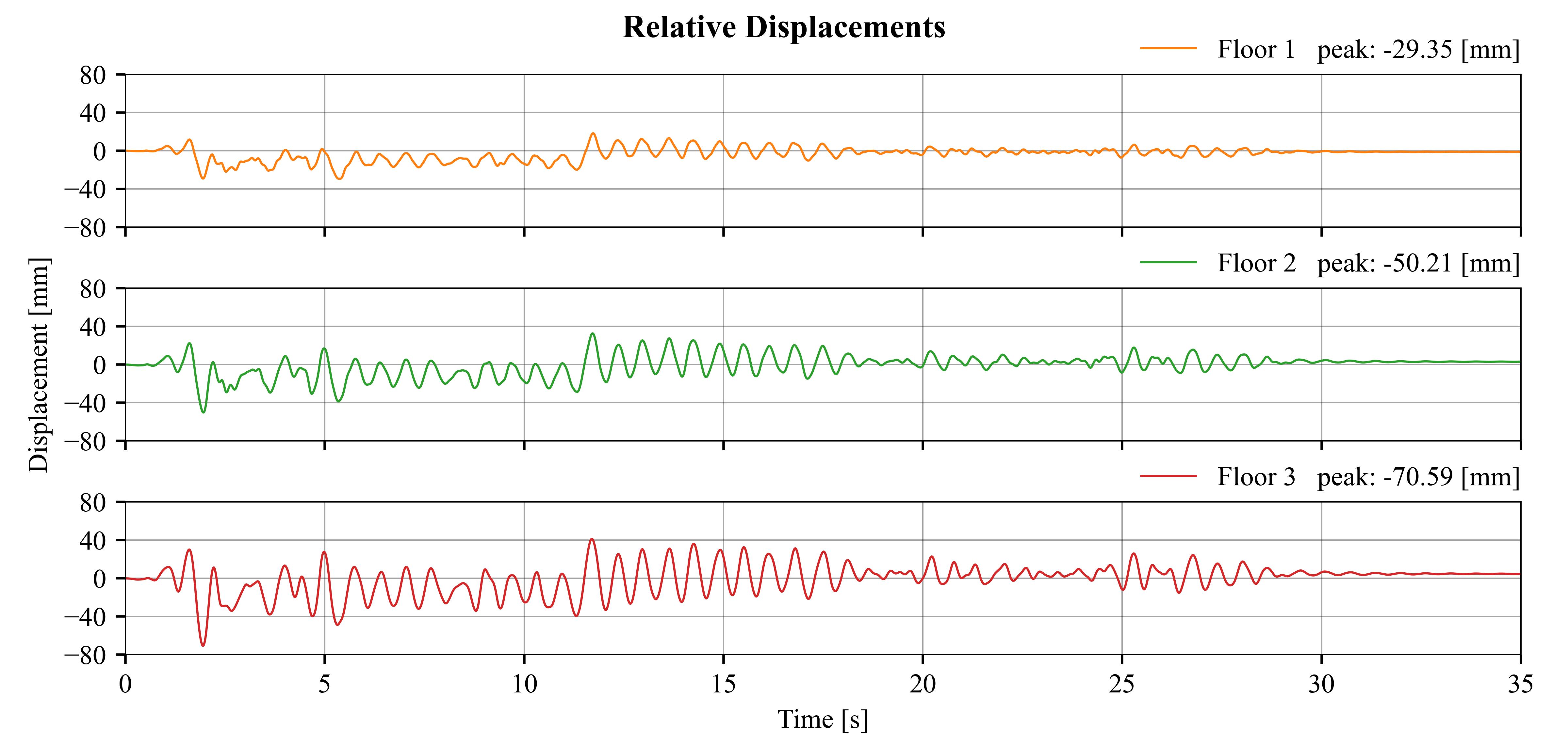
89rD_path = r'./Relative_disp.out'
90ops.recorder('Node', '-file', r'./Relative_disp.out', '-time', '-dT', dt_out, '-node', 1, 2, 3, '-dof', 1, 'disp') # Relative displacements with respect to the ground
91
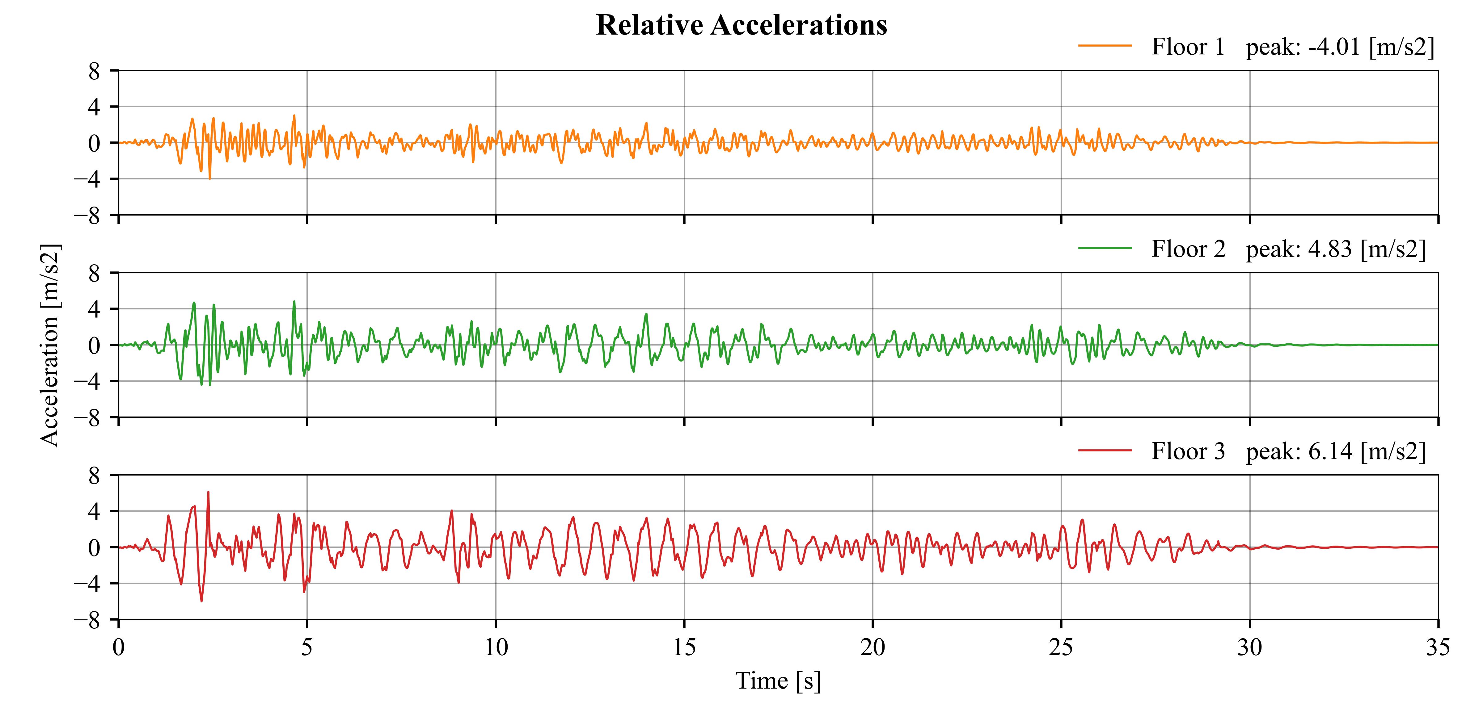
92rA_path = r'./Relative_accel.out'
93ops.recorder('Node', '-file', rA_path, '-time', '-dT', dt_out, '-node', 1, 2, 3, '-dof', 1, 'accel') # Relative accelerations with respect to the ground
94
95aA_path = r'./Absolute_accel.out'
96ops.recorder('Node', '-file', aA_path, '-timeSeries', load_tag, '-time', '-dT', dt_out, '-node', 0, 1, 2, 3, '-dof', 1, 'accel') # Absolute accelerations
97
98eF_path = r'./Element_force.out'
99ops.recorder('Element', '-file', eF_path, '-time', '-dT', dt_out, '-ele', 1, 2, 3, 'localForce') # Local spring force
100
101# Run the dynamic analysis
102Gamma = 0.5
103Beta = 0.25
104tol = 1.0e-12
105itrs = 100
106ops.wipeAnalysis()
107ops.algorithm('Newton')
108ops.system('BandGen')
109ops.numberer('Plain')
110ops.constraints('Plain')
111ops.integrator('Newmark', Gamma, Beta)
112ops.analysis('Transient')
113ops.test('NormUnbalance', tol, itrs)
114num_steps = int(tFinal/dt_out+1)
115ops.analyze(num_steps, dt_out)
116ops.wipe()
117
118rD = np.genfromtxt(rD_path, usecols=[1, 2, 3]).T
119
120rA = np.genfromtxt(rA_path, usecols=[1, 2, 3]).T
121aA = np.genfromtxt(aA_path, usecols=[1, 2, 3, 4]).T
122
123eF = np.genfromtxt(eF_path, usecols=[1, 2, 3]).T
124
125
126# Matplotlib plots
127rD /= mm
128K = [K1, K2, K3]
129Py = [Py1, Py2, Py3]
130plot_nonlinear_mdof_graphs.plot(N, rD, rA, aA, eF, dt_out, num_steps, tFinal, K, Py)